EXCEL: How to Make a Drop-Down List Change Depending on Selection in Different List

• Open Excel
• Click on a New Sheet
• The Following Data (no heading, no blank rows and no blank columns in the table)

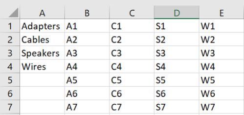
• These products have 4 products and the styles are in the following columns to represent each product. Foe example: Speakers contain S1 through S7 styles.
• Highlight the 4 products and name them through the Formula Tab and in the Define Names Group, use the Define name command (no spaces in the name). I called it ProductCategories
• Go back to sheet 1 and do not place column heading names yet
• Highlight several cells in column A to start the drop-down list
• Click Data tab, Data Validation, Data Validation, choose List from the Allow: drop down list
• Enter =ProductCategories in the Source area and hit OK
• Select the same number of cells like in Column A in Column B
• Click Data tab, Data Validation, Data Validation, choose List from the Allow: drop down list
• Enter =indirect(A1) in the Source area and hit Ok
• Try it out! If you select Speakers in Column A then in Column B, only the choices will be S1 through S7
• Why does it work? The answer is simple.  Since we have 4 product, the next 4 columns must be with data.  Since Speakers is third choice, Excel will count 3 columns after Column A.

Here is the file.  First sheet called choice has the drop down choices that work. An the Product sheet lists the products and the subcategories for each product.

How to Make a Drop and Multiple Selections

EXCEL: Quick Method for Frequency

We can use the Frequency formula when there are multiple columns to compile.  If you have just have one column, you can use the Data Analysis in the Analyze group under the Data tab to perform the frequency.

Step 1: If you do not see this on the menu

1. In the Backstage view, Click Options
2. Click Add-ins
3. In the Manage list, click Excel Add-ins, then click Go.
4. Check Analysis ToolPak, then click OK
5. After loading the Toolpak add-in, there will be an Analysis group on the Data tab, with a Data Analysis.

Step 2: Using Histogram to perform the frequency

1. The input should be a single set of data
2. The bins should be the bands you want to use for the frequncy
3. Click Data Analysis,  then select Histogram and click OK
4. Specify the data range and the bins
5. Select where you want to place the output

The output is as follows:

If you want to add a Histogram chart then select in the dialogue box–> Chart Output.  The result is as follows:

See January 31, 2013 blog for advanced Frequency command.

Enjoy!

EXCEL: Entering Info Without Moving to Next Cell

As Excel users, we were taught that you enter information in the cell and hit Enter.  This actions navigates to the next cell below. It is in the File Options that sets up it to automatically moves down to the next cell when you Enter.  Guess what, if you hit Control+Enter, the information is enter and it REMAINS in that cell. It does not navigate down to the next cell.

Enjoy

Excel: Clean and Reformat Telephone Numbers

I am recently working on a project where there are some many different formats of telephone numbers in one column that I needed to clean  it up.  Well, I found a site called ExcelJet that supplied the formula called Substitute and the explanation.

How this formula works

The formula runs from the inside out, with each SUBSTITUTE removing one character.

The inner most SUBSTITUTE removes the left parentheses, and the result is handed to the next SUBSTITUTE, which removes the right parentheses, and so on.

Whenever you use the SUBSTITUTE function, the result will be text. Because you can’t apply a number format to text, we need to convert the text to a number. One way to do that is to add zero (+0), which automatically converts numbers in text format to numbers in numeric format.

Finally, the “Special” telephone number format is applied (column D).

White space trick for better readability

When nesting multiple functions, it can be difficult to read the formula and keep all parentheses balanced. Excel doesn’t care about extra white space in a formula, so you can add line breaks in the formula to make the formula more readable. For example, the formula above can be written as follows:

=SUBSTITUTE(
SUBSTITUTE(
SUBSTITUTE(
SUBSTITUTE(
SUBSTITUTE(
A1,
“(“,””),
“)”,””),
“-“,””),
” “,””),
“.”,””)

Note that the cell appears in the middle, with function names above and substitutions below. Not only does this make the formula easier to read, it also makes it easier to add and remove substitutions.

Just remember that you have to copy the new results in a blank column as Paste Values Only!!

You can use this same trick to make nested IF statements easier to read as well.

Thank You ExcelJet!

Excel-Repeat Data to Selected Cells

What a great trick to use in Excel.  Select several blank cells. Type what you want to repeat in those selected cells and hit Control+Enter keys.  The information is entered in all of the selected cells. This eliminates you to type in one cell and then to use the autofill function.

Enjoy!

EXCEL: Using Convert Formula

To convert miles to kilometers:

1. Select cell E5 and type =CONVERT(. or Click on Formulas Tab, More Functions, Engineering, Convert)
2. Click the Paste Function button to access the Function Arguments window.
3. Select cell D5, which holds the value you wish to convert, so the cell reference appears in the Number text box.
4. Press [Tab] and enter mi in the From_Unit text box.
5. Press [Tab], enter km in the To_Unit text box, and click OK.
6. Select cell E5 and drag its fill handle down to cell E9 to apply the formula to the other cells.
7. Select the range E5:E9 and click the Decrease Decimal button on the Formatting toolbar until the values display in tenths of a kilometer.

The CONVERT function also converts units of measurement for mass, pressure, liquid, and many others. For a complete list, along with the unit abbreviations accepted by the function, type CONVERT in Excel’s Help window.

Once you create a worksheet based on our example, you can use the CONVERT function to instantly perform the conversions from miles to kilometers.

EXCEl: 300 Formula Examples

I was teaching my Computer Literacy class and the students wanted me to give examples of different formulas.  Thank goodness for the internet because I found a site that links to over 300 Excel formula examples. This site created by EXCELJET.com allows you to click on a formula for a full description as well as an excel example. Related functions appear to the right and are also clickable. Also click “list of Excel functions” to see the list of functions. You can also search for a function as well. Here is the URL for you to copy and paste in your browser:

https://exceljet.net/formulas

 

WORD: Creating Beautiful Font

If you want to design a beautiful font like the image here, there are the steps in Word:

Steps:

1. Highlight the words and change font to Gabriola.
2. Click on the Font dialogue box launcher (little box with arrow–bottom righ corner of the font group).
3. From the Ligatures box, choose Historical and Discretionary.
4. From the Number spacing box, choose Default.
5. From the Number forms box, choose Old-stlye.
6. From the Stylistic sets box, choose 6.
7. Make sure the paragraph is double space as well.

WORD, EXCEL, PPT: Creating Hyperlinks

How To Insert Hyperlinks

Hyperlinks add the capability of moving from one position to another quickly and easily, such as linking to another slide, another file, or even to a web site.

1. Highlight the text or graphics to link
2. Insert Tab > Links command group > Hyperlink
3. Choose the target (Place in this document)
4. Choose the slide

Once a link has been followed, the linked text will change color. You may want to create a “Return” hyperlink.

One advantage of hyperlinking to a separate file is that the size of the presentation file remains smaller than if the file was inserted into the presentation. A disadvantage of linking separate files is that if the name of the linked document changes or if it is moved into a different directory, the link will be broken and the information will not be accessible.

EXCEL: Comparing Two Columns

Did you know that you can use the Go To Special command to help you compare two columns? This command identifies the differences quickly.  Here are the steps:

1. Select the column you want to find the differences.
2. Use the Ctrl key to select the original column.
3. On the Home tab, select Find & Replace, Go To Special, check Row Differences and click Ok.

The items in the difference column will be highlighted for you.

Then select the red font color in order for you to see the differences between the column.